Dynamic Programming
#RL #Learning #computer-science #Control
The term dynamic programming (DP) refers to a collection of algorithms that can be used to compute optimal policies given a perfect model of the environment as a Markov decision process (MDP). In this note we learn how DP algorithms use the value function to search for better policies.
Policy Evaluation
Assume you are given an arbitrary policy $\pi$. How would you compute the state-value function $v_\pi (s)$? This is called policy evaluation in the DP literature. We also refer to it as the prediction problem. Remember that for all $s \in \mathcal{S}$, we have \(v_\pi (s) = \mathbb{E}_\pi \{ R_{t + 1} + \gamma R_{t + 2} + \gamma^2 R_{t + 3} + \ldots \ | \ S_t = s \} =\) \(\mathbb{E}_\pi \{ R_{t + 1} + \gamma v_\pi (S_{t + 1}) \ | \ S_t = s \}\) \(\sum_a \pi (a \ | \ s) \sum_{s', r} p(s', r \ | \ s, a) [r + \gamma v_\pi (s')]\) If the environment’s dynamics are completely known, then this is a system of $|\mathcal{S}|$ simultaneous linear equations in $|\mathcal{S}|$ unknowns, but this is very computationally exhaustive. Iterative solution methods also exist. Consider a sequence of approximate value functions $v_0, v_1, v_2, \ldots$, each mapping $\mathcal{S}^+$ to $\mathbb{R}$. The initial approximation, $v_0$, is chosen arbitrarily (except that the terminal state, if any ,must be given value $0$), and each successive approximation is obtained by using the Bellman equation for $v_\pi$ as an update rule: \(v_{k + 1} (s) = \mathbb{E}_\pi [R_{t + 1} + \gamma v_k (S_{t + 1}) \ | \ S_t = s] =\) \(\sum_a \pi (a \ | \ s) \sum_{s', r} p(s', r \ | \ s, a) [r + \gamma v_k (s')]\) for all $s \in \mathcal{S}$. Clearly, $v_k = v_\pi$ is a fixed point for this update rule. The sequence ${ v_k }$ can be shown in general to converge to $v_\pi$ as $k \rightarrow \infty$ under the same conditions that guarantee the existence of $v_\pi$. This algorithm is called iterative policy evaluation. Note that this algorithm applies the same operation to each state $s$ and replaces it with a new value obtained from the old values of the successor states of $s$. This is called a full backup. Also, instead of using the old values on the right, we could update the states in a sweep and use new values on the right, wherever they are available. This method can be shown to also converge to $v_\pi$, and is usually faster. The iterative procedure only stops in the limit. A typical stopping condition for iterative policy evaluation is to test the quantity $\max_{s \in \mathcal{S}} |v_{k + 1} (s) - v_k (s)|$after each sweep and stop when it is sufficiently small.
Policy Improvement
Assume that you have a policy $\pi$ and you would like to know if for a state $s$, there is an action $a \neq \pi(s)$ that performs better than policy $\pi$ would have. One way to answer that would be to check the action-value function: \(q_\pi (s, a) = \mathbb{E}_\pi [R_{t + 1} + \gamma v_\pi (S_{t + 1}) \ | \ S_t = s , A_t = a] = \sum_{s', r} p(s', r \ | \ s, a) [r + \gamma v_\pi (s')]\) The key criterion is whether this is greater than or less than $v_\pi (s)$. This is a special case of the policy improvement theorem.
policy improvement theorem: Let $\pi$ and $\pi’$ be any pair of deterministic policies such that, for all $s \in \mathcal{S}$, \(q_\pi (s, \pi' (S)) \geq v_\pi (s)\) Then the policy $\pi’$ must be as good as or better than policy $\pi$. That is, it must obtain greater or equal expected return from all states $s \in \mathcal{S}$: \(v_{\pi'} (s) \geq v_\pi (s)\) Moreover, if there is strict inequality in the first equation at any state, then there must be strict inequality in the second equation at at least one state.
We can use the policy improvement theorem to construct a policy $\pi’$ given policy $\pi$, ensuring that $\pi’ \geq \pi$. \(\pi' (s) = arg \max_a q_\pi (s, a) = arg \max_a \mathbb{E} [R_{t + 1} + \gamma v_\pi (S_{t + 1}) \ | \ s_t = s, A_t = a] =\) \(arg \max_a \sum_{s', r} p(s', r \ | \ s, a) [r + \gamma v_\pi (s')]\) The process of making a new policy that improves on an original policy, by making it greedy with respect to the value function of the original policy, is called policy improvement. Policy improvement gives a strictly better policy except when the original policy is already optimal. If there are ties in policy improvement steps ,that is, if there are several actions at which the maximum is achieved, then in the stochastic case we need not select a single action from among them. Instead, each maximizing action can be given a portion of the probability of being selected in the new greedy policy. Any apportioning scheme is allowed as long as all submaximal actions are given zero probability.
Policy Iteration
Policy iteration is a way of finding an optimal policy. For a policy $\pi$, we use policy evaluation to find $v_\pi$ and then we use policy improvement to find a better policy $\pi’$. Then, again, we use policy evaluation to find $v_{\pi’}$ and so on.

This process must converge to an optimal policy and optimal value function in a finite number of iterations. Also, the policy evaluation step is usually started with the value function for the previous policy. This typically results in a great increase in the speed of convergence of policy evaluation.
Value Iteration
Each step of the policy iteration method is an iterative procedure itself, which could cause the algorithm to be computationally exhaustive. The policy evaluation step of policy iteration can be truncated in several ways without losing the convergence guarantees of policy iteration. One important special case is when policy evaluation is stopped after just one sweep (one backup of each state). This algorithm is called value iteration. Value iteration can be shown in a single mathematical equation as \(v_{k + 1} (s) = \max_a \mathbb{E} [R_{t + 1} + \gamma v_\k (S_{t + 1}) \ | \ S_t = s, A_t = a] = \max_a \sum_{s', r} p(s', r \ | \ s, a) [r + \gamma v_k (s')],\) for all $s \in \mathcal{S}$. For arbitrary $v_0$, the sequence ${ v_k }$ can be shown to converge to $v_\ast$ under the same conditions that guarantee the existence of $v_\ast$. Note that value iteration is obtained simply by turning the Bellman optimality equation into an update rule. Value iteration effectively combines, in each of its sweeps, one sweep of policy evaluation and one sweep of policy improvement.
Asynchronous Dynamic Programming
A major drawback to the DP methods that we have discussed so far is that they require sweeps of the state set. If the state set is very large, this can be very expensive. Asynchronous DP algorithms are in-place iterative DP algorithms that are not organized in terms of systematic sweeps of the state set. These algorithms back up the values of states in any order whatsoever, using whatever values of other states happen to be available. To converge correctly, however, an asynchronous algorithm must continue to backup the values of all the states: it can’t ignore any state after some point in the computation. Of course, avoiding sweeps does not necessarily mean that we can get away with less computation. It just means that an algorithm does not need to get locked into any hopelessly long sweep before it can make progress improving a policy.
Generalized Policy Iteration
Policy iteration consists of two simultaneous, interacting processes:
- policy evaluation: making the value function consistent with the current policy
- policy improvement: making the policy greedy with respect to the current value function
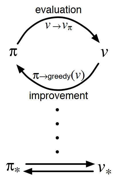
We use the term generalized policy iteration (GPI) to refer to the general idea of letting policy evaluation and policy improvement processes interact.
Note that if both the evaluation process and the improvement process stabilize, that is, no longer produce changes, then the value function and policy must be optimal. The value function stabilizes only when it is consistent with the current policy, and the policy stabilizes only when it is greedy with respect to the current value function. Thus, both processes stabilize only when a policy has been found that is greedy with respect to its own evaluation function. This implies that the Bellman optimality equation holds.
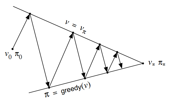
The evaluation and improvement processes in GPI can be viewed as both competing and cooperating. They compete in the sense that they pull in opposing directions. Making the policy greedy with respect to the value function typically makes the value function incorrect for the changed policy, and making the value function consistent with the policy typically causes that policy no longer to be greedy. In the long run, however, these two processes interact to find a single joint solution: the optimal value function and an optimal policy.
Efficiency of Dynamic Programming
A DP method is guaranteed to find an optimal policy in polynomial time even though the total number of (deterministic) policies is $m^n$ ($n$ and $m$ denote the number of states and actions).. In this sense, DP is exponentially faster than any direct search in policy space could be. DP is sometimes thought to be of limited applicability because of the curse of dimensionality. Large state sets do create difficulties, but these are inherent difficulties of the problem, not of DP as a solution method.
Finally note that all DP methods update estimates of the values of states based on estimates of the values of successor states. That is, they update estimates on the basis of other estimates. This general idea is called bootstrapping.
Continue reading about reinforcement learning here.
Sources: